A drawback of the VLOOKUP function is that it can only look up values in the leftmost column of a table. However, sometimes you need to look up a value in any column and return the corresponding value to the left. To achieve this, simply use the INDEX and the MATCH function.
1. The MATCH function returns the position of a value in a given range.
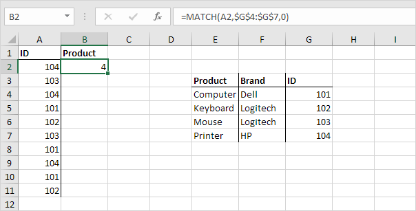
Explanation: 104 found at position 4 in the range $G$4:$G$7.
2. Use this result and the INDEX function to return the 4th value in the range $E$4:$E$7.

3. Drag the formula in cell B2 down to cell B11.

Note: when we drag this formula down, the absolute references ($E$4:$E$7 and $G$4:$G$7) stay the same, while the relative reference (A2) changes to A3, A4, A5, etc
0 comments:
Post a Comment